
Image Super-Resolution using Generative Models on the SEN2VENµS Dataset
Author
- Debwashis Borman
Dataset
I used the SEN2VENµS dataset, which is designed specifically for super-resolution in remote sensing.
It provides paired Sentinel-2 and VENµS observations across 29 global sites.
For my experiments, I picked 6 representative sites:
- ALSACE (France, Alsace)
- ANJI (China, Zhejiang Sheng)
- BENGA (India, West Bengal)
- LERIDA-1 (Spain, Catalonia)
- NARYN (Kyrgyzstan, Naryn)
- SO2 (France, Midi-Pyrénées)
To make the evaluation fair, I split the data by site (so there’s no spatial overlap):
- Train: 12,355 pairs (~70%)
- Validation: 2,649 pairs (~15%)
- Test: 2,650 pairs (~15%)
Tasks I worked on:
- 2× Super-Resolution
- Input: Sentinel-2 RGBI bands (10m)
- Target: VENµS (5m)
- 4× Super-Resolution
- Input: Sentinel-2 Red Edge bands (20m)
- Target: VENµS (5m)
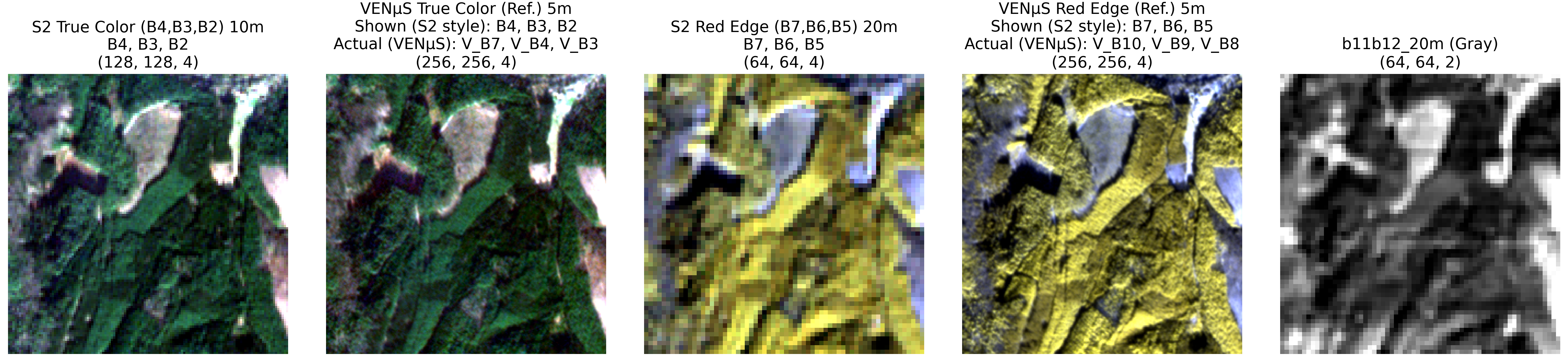 Data Visualization after extraction and Processing
Models
I compared both classical deep SR models and GAN-based approaches:
-
SRCNN
The first CNN for super-resolution. Very simple 3-layer design – works better than bicubic, but tends to blur fine details. -
RCAN
A much deeper CNN with attention modules. This one is great at preserving structure and sharpness, and usually gives the best scores. -
ESRGAN
A GAN-based model that focuses on realism and textures. It uses Residual-in-Residual Dense Blocks (RRDB) and a perceptual loss based on VGG19 features.
It often produces visually sharper results, though sometimes at the cost of pixel-accuracy.
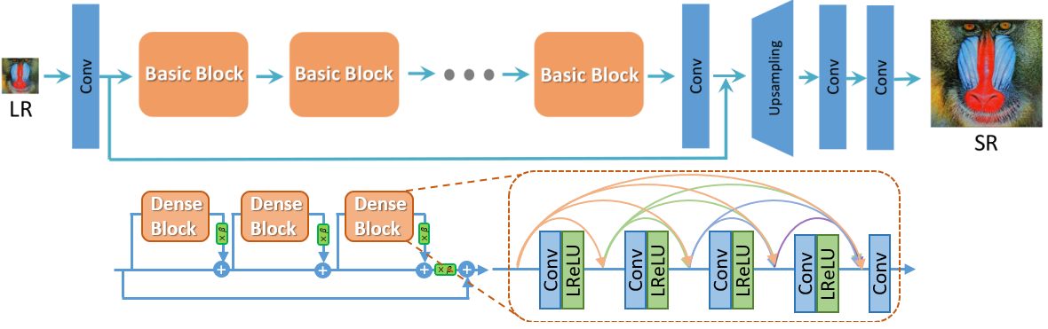 ESRGAN Architecture
Results
I evaluated the models in two ways:
- Quantitatively using PSNR, SSIM, and LPIPS
- Qualitatively by visually comparing cropped regions
Quantitative Results
2× SR (Sentinel-2 RGBI → VENµS 5m)
| Model | PSNR | SSIM | LPIPS (RGB) | LPIPS (NIRG) |
|---|---|---|---|---|
| SRCNN | 38.39 | 0.960 | 0.095 | 0.133 |
| RCAN | 42.32 | 0.981 | 0.056 | 0.079 |
| ESRGAN | 37.45 | 0.950 | 0.085 | 0.152 |
4× SR (Sentinel-2 Red Edge → VENµS 5m)
| Model | PSNR | SSIM | LPIPS (567) | LPIPS (678) |
|---|---|---|---|---|
| SRCNN | 34.71 | 0.903 | 0.294 | 0.248 |
| RCAN | 37.36 | 0.936 | 0.178 | 0.155 |
| ESRGAN | 37.51 | 0.928 | 0.177 | 0.154 |
| ESRGAN (8ch) | 36.38 | 0.925 | 0.279 | 0.345 |
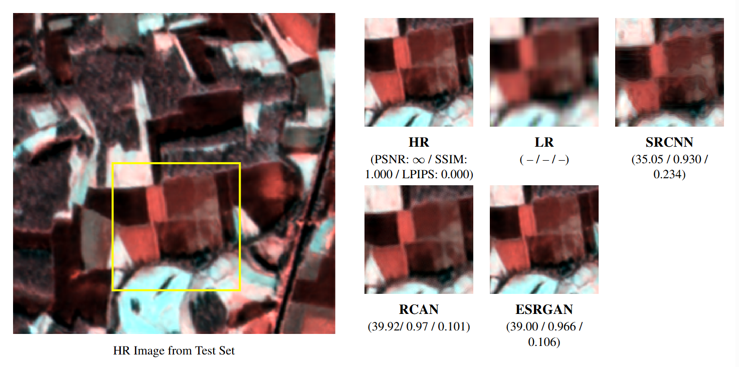
Qualitative Results
2× RGB bands:
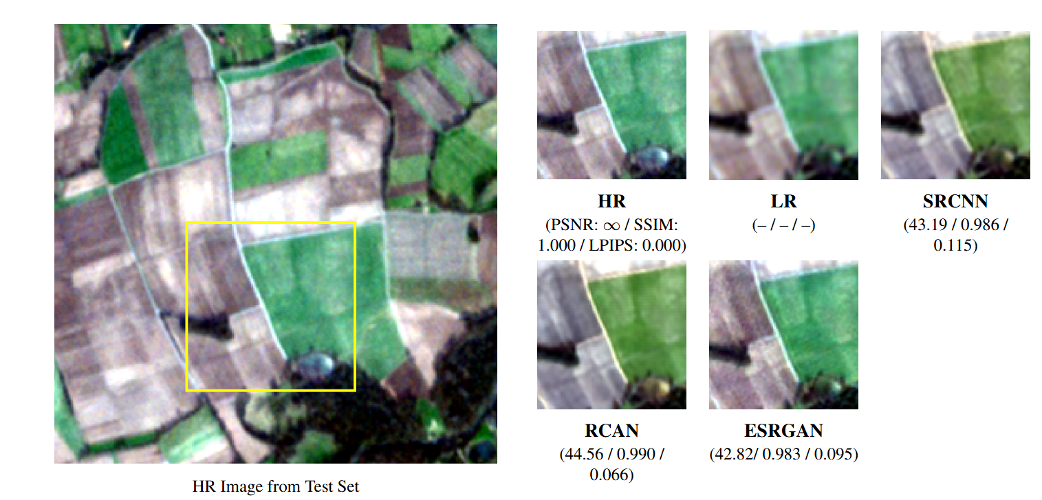 HR with ROI (left) and crops from HR, LR, SRCNN, RCAN, ESRGAN (right).
2× NIRG bands:
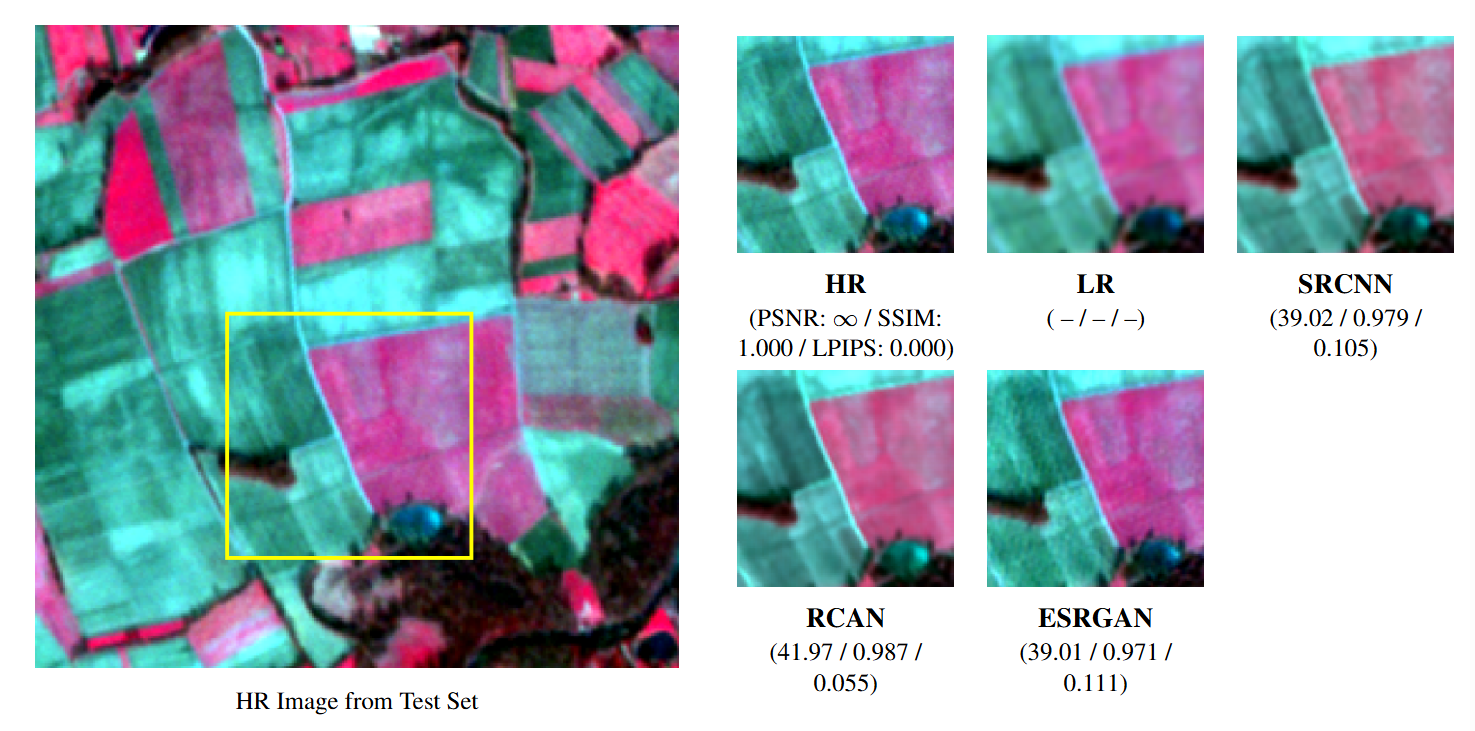 Comparison on NIRG bands.
4× Red Edge (5-6-7 bands):
 Comparison on 5-6-7 bands.
Observations
- RCAN is the most reliable when it comes to numerical accuracy (best PSNR/SSIM and lowest LPIPS).
- ESRGAN produces sharper and more realistic textures, making the images “look” better, even if the scores are a bit lower.
- SRCNN is a solid baseline, but clearly outdated compared to the other two.
Final Note
This project was a great learning experience – from handling multispectral remote sensing data to adapting GANs for SR tasks.
As the sole author, I built everything from dataset preparation to model training and evaluation, and I’m excited to share the results here.